CAM and SeCAM: Explainable AI for Understanding Image Classification Models
Introduction
Explainable Artificial Intelligence (XAI) has emerged as a crucial aspect of AI research, aiming to enhance the transparency and interpretability of AI models. Understanding the decision-making process of AI systems is essential for ensuring trust, accountability, and safety in their applications. In this tutorial, we focus on Class Activation Mapping (CAM) and Segmentation Class Activation Mapping (SeCAM). Specifically, we consider their application in explaining the decisions of the ResNet50 model, a pivotal architecture within the domain of deep CNNs that has significantly impacted image classification tasks. CAM and SeCAM in particular aim to provide fast and intuitive explanations by identifying image regions most influential to the model’s prediction.
Section 1: Overview of XAI Methods
Explainable AI (XAI) refers to methods and techniques in the application of artificial intelligence technology such that the results of the solution can be understood by human experts. It contrasts with the concept of the “black box” in machine learning where even their designers cannot explain why the AI arrived at a specific decision. XAI is becoming increasingly important as AI systems are used in more critical applications such as diagnostic healthcare, autonomous driving, and more.
Section 2: ResNet50 Architecture and Importance of Understanding
The ResNet50 model is a pivotal architecture within the domain of deep convolutional neural networks (CNNs) that has significantly impacted image classification tasks, notably achieving remarkable success in the ImageNet Large Scale Visual Recognition Challenge (ILSVRC). Generally, ResNet50 has the following architecture:

The ResNet50 model, while renowned for its high accuracy in image classification tasks, exemplifies the “black box” nature inherent to many advanced deep learning models. This characteristic poses a significant challenge for AI researchers, practitioners, and end-users who seek to understand the model’s predictive behaviour. The intricate architecture of ResNet50, characterised by its deep layers and residual blocks, complicates the interpretation of how input features influence the final classification outcomes
Section 3: Class Activation Mapping (CAM)
General Definition
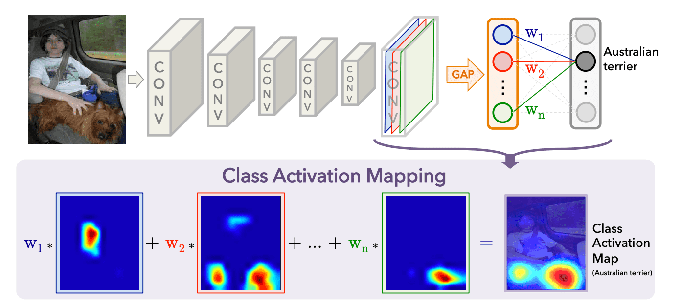
Class Activation Mapping (CAM) is a technique used to identify the discriminative regions in an image that contribute to the class prediction made by a Convolutional Neural Network (CNN). CAM is particularly useful for understanding and interpreting the decisions of CNN models.
How CAM Works:
a) Steps Involved in CAM:
- Feature Extraction:
- Extract the feature maps from the last convolutional layer of the CNN.
- Global Average Pooling (GAP):
- Apply Global Average Pooling (GAP) to the feature maps to get a vector of size equal to the number of feature maps.
- Fully Connected Layer:
- The GAP output is fed into a fully connected layer to get the final class scores.
- Class Activation Mapping:
- For a given class, compute the weighted sum of the feature maps using the weights from the fully connected layer.
b) Equations
- Feature Maps:
- Let $f_k(x, y)$ represent the activation of unit $k$ in the feature map at spatial location $(x, y)$.
- Global Average Pooling:
- The GAP for feature map $k$ is computed as: $F_k = \frac{1}{Z} \sum_{x} \sum_{y} f_k(x, y)$ where $Z$ is the number of pixels in the feature map.
- Class Score:
- The class score $S_c$ for class $c$ is computed as: $S_c = \sum_{k} w_{k}^{c} F_k $ where $w_{k}^{c}$ is the weight corresponding to class $c$ for feature map $k$.
- Class Activation Map:
- The CAM for class $c$ is computed as: $M_c(x, y) = \sum_{k} w_{k}^{c} f_k(x, y)$ This gives the importance of each spatial element $(x, y)$ in the feature maps for class $c$.
c) Implementation with Code
Step 1: Preprocess the Input Image
Firstly, we need to read and preprocess the input image to make it compatible with the ResNet50 model. The preprocessing steps include resizing the image to 224x224 pixels, normalizing it, and converting it to a PyTorch tensor.
def preprocess_image(image_path):
    """
    Preprocess the input image.
    :param image_path: Path to the input image
    :return: Preprocessed image tensor, original image, image dimensions
    """
    image = cv2.imread(image_path)
    original_image = image.copy()
    image = cv2.cvtColor(image, cv2.COLOR_BGR2RGB)
    height, width, _ = image.shape

    preprocess = transforms.Compose([
        transforms.ToPILImage(),
        transforms.Resize((224, 224)),
        transforms.ToTensor(),
        transforms.Normalize(mean=[0.485, 0.456, 0.406], std=[0.229, 0.224, 0.225])
    ])

    image_tensor = preprocess(image)
    image_tensor = image_tensor.unsqueeze(0)
    return image_tensor, original_image, height, width
image = cv2.imread(image_path): Reads the image from the specified path using OpenCV.original_image = image.copy(): Creates a copy of the original image to preserve it for later use.image = cv2.cvtColor(image, cv2.COLOR_BGR2RGB): Converts the image from BGR to RGB format as OpenCV reads images in BGR format by default.height, width, _ = image.shape: Retrieves the dimensions (height and width) of the image.preprocess = transforms.Compose([...]): Defines a series of preprocessing steps:transforms.ToPILImage(): Converts the image to PIL format.transforms.Resize((224, 224)): Resizes the image to 224x224 pixels.transforms.ToTensor(): Converts the image to a PyTorch tensor.transforms.Normalize(mean=[0.485, 0.456, 0.406], std=[0.229, 0.224, 0.225]): Normalizes the image tensor using the specified mean and standard deviation.
image_tensor = preprocess(image): Applies the preprocessing steps to the image.image_tensor = image_tensor.unsqueeze(0): Adds a batch dimension to the image tensor, making it compatible for input to the CNN.
Step 2: Load Model and Extract Features
Secondly, we need to load a pre-trained ResNet50 model and extract the feature maps from the last convolutional layer.
def load_model_and_extract_features():
    """
    Load the pretrained ResNet50 model and extract features.
    :return: Model, features blob list, softmax weights
    """
    model = models.resnet50(weights=models.ResNet50_Weights.DEFAULT).eval()
    features_blobs = []

    def hook_feature(module, input, output):
        features_blobs.append(output.data.cpu().numpy())

    # Hook the feature extractor to get the convolutional features from 'layer4'
    model._modules.get('layer4').register_forward_hook(hook_feature)

    # Get the softmax weights
    params = list(model.parameters())
    softmax_weights = np.squeeze(params[-2].data.numpy())

    return model, features_blobs, softmax_weights
model = models.resnet50(weights=models.ResNet50_Weights.DEFAULT).eval(): Loads a pre-trained ResNet50 model and sets it to evaluation mode.features_blobs = []: Initializes an empty list to store feature maps from the hooked layer.def hook_feature(module, input, output): Defines a hook function that captures the output of the specified layer.features_blobs.append(output.data.cpu().numpy()): Appends the output feature maps to thefeatures_blobslist, converting them to NumPy arrays and moving them to the CPU.model._modules.get('layer4').register_forward_hook(hook_feature): Registers the hook on the last convolutional layer (layer4) of the model to capture its output.params = list(model.parameters()): Retrieves the parameters of the model.softmax_weights = np.squeeze(params[-2].data.numpy()): Extracts and squeezes the softmax weights from the fully connected layer of the model, converting them to a NumPy array.
Step 3: Get Top K Predictions
Thirdly, we need to perform a forward pass through the model, compute the softmax probabilities, and retrieve the top K class indices with the highest probabilities.
def get_topk_predictions(model, image_tensor, topk_predictions):
    """
    Get the top k predictions for the input image.
    :param model: Pretrained model
    :param image_tensor: Preprocessed image tensor
    :param topk_predictions: Number of top predictions to get
    :return: Top k class indices
    """
    outputs = model(image_tensor)
    probabilities = F.softmax(outputs, dim=1).data.squeeze()
    class_indices = topk(probabilities, topk_predictions)[1].int()
    return class_indices
outputs = model(image_tensor): Performs a forward pass through the model using the preprocessed image tensor.probabilities = F.softmax(outputs, dim=1).data.squeeze(): Computes the softmax probabilities for the outputs, normalizing them across the class dimension, and removes extra dimensions.class_indices = topk(probabilities, topk_predictions)[1].int(): Retrieves the indices of the top K classes with the highest probabilities using thetopkfunction.
Step 4: Generate Class Activation Maps (CAM)
After all the above steps, we can generate the Class Activation Maps (CAM) for the top K predictions.
def generate_CAM(feature_maps, softmax_weights, class_indices):
    """
    Generate Class Activation Maps (CAM).
    :param feature_maps: Convolutional feature maps
    :param softmax_weights: Weights of the fully connected layer
    :param class_indices: Class indices
    :return: List of CAMs for the specified class indices
    """
    batch_size, num_channels, height, width = feature_maps.shape
    output_cams = []

    for class_idx in class_indices:
        cam = softmax_weights[class_idx].dot(feature_maps.reshape((num_channels, height * width)))
        cam = cam.reshape(height, width)
        cam = cam - np.min(cam)  # Normalize CAM to be non-negative
        cam = cam / np.max(cam)  # Scale CAM to be in range [0, 1]
        cam_img = np.uint8(255 * cam)  # Convert to uint8 format
        output_cams.append(cam_img)

    return output_cams
batch_size, num_channels, height, width = feature_maps.shape: Retrieves the shape of the feature maps.output_cams = []: Initializes an empty list to store the CAMs.for class_idx in class_indices: Iterates over each class index.cam = softmax_weights[class_idx].dot(feature_maps.reshape((num_channels, height * width))): Computes the CAM by taking the weighted sum of the feature maps.cam = cam.reshape(height, width): Reshapes the CAM to the original feature map size.cam = cam - np.min(cam): Normalizes the CAM to be non-negative.cam = cam / np.max(cam): Scales the CAM to be in the range [0, 1].cam_img = np.uint8(255 * cam): Converts the CAM to uint8 format.output_cams.append(cam_img): Adds the CAM to the list of output CAMs.
This function computes the CAM for each class index by taking the weighted sum of the feature maps using the softmax weights. It normalizes and converts the CAM to an 8-bit image.
Step 5: Display and Save the CAM
After generating the CAMs, we can overlay them on the original image and display the results.
def display_and_save_CAM(CAMs, width, height, original_image, class_indices, class_labels, save_name, plot=True):
    """
    Display and save the CAM images.
    :param CAMs: List of CAMs
    :param width: Width of the original image
    :param height: Height of the original image
    :param original_image: Original input image
    :param class_indices: Class indices
    :param class_labels: List of all class names
    :param save_name: Name to save the output image
    :param plot: Whether to display the image
    """
    matplotlib.rcParams['figure.figsize'] = 15, 12

    for i, cam in enumerate(CAMs):
        heatmap = cv2.applyColorMap(cv2.resize(cam, (width, height)), cv2.COLORMAP_JET)
        result = heatmap * 0.3 + original_image * 0.5
        # Put class label text on the result
        cv2.putText(result, class_labels[class_indices[i]], (20, 40),
                    cv2.FONT_HERSHEY_SIMPLEX, 1.5, (0, 255, 0), 2)
        cv2.imwrite(f"outputs/CAM_{save_name}_{i}.jpg", result)

        # Display the result
        if plot:
            image = plt.imread(f"outputs/CAM_{save_name}_{i}.jpg")
            plt.imshow(image)
            plt.axis('off')
            plt.show()
matplotlib.rcParams['figure.figsize'] = 15, 12: Sets the figure size for matplotlib plots.for i, cam in enumerate(CAMs): Iterates over each CAM.heatmap = cv2.applyColorMap(cv2.resize(cam, (width, height)), cv2.COLORMAP_JET): Creates a heatmap by resizing the CAM and applying a colormap.result = heatmap * 0.3 + original_image * 0.5: Overlays the heatmap on the original image.cv2.putText(result, class_labels[class_indices[i]], (20, 40), cv2.FONT_HERSHEY_SIMPLEX, 1.5, (0, 255, 0), 2): Adds the class label to the result image.cv2.imwrite(f"outputs/CAM_{save_name}_{i}.jpg", result): Saves the result image.image = plt.imread(f"outputs/CAM_{save_name}_{i}.jpg"): Reads the saved image.plt.imshow(image): Displays the image.plt.axis('off'): Hides the axis.plt.show(): Shows the image.
This function overlays the CAM on the original image, adds the class label, and saves the result. It also displays the final image.
Step 6: Full Pipeline for Generating and Saving CAM
Finally, we can combine all the above steps into a single function to generate and save CAMs for the top K predictions of an input image.
def generate_and_save_CAM(image_path, topk_predictions):
    """
    Generate and save CAM for the specified image and topk predictions.
    :param image_path: Path to the input image
    :param topk_predictions: Number of top predictions to generate CAM for
    """
    # Load the class labels
    class_labels = load_class_labels('LOC_synset_mapping.txt')

    # Read and preprocess the image
    image_tensor, original_image, height, width = preprocess_image(image_path)

    # Load the model and extract features
    model, features_blobs, softmax_weights = load_model_and_extract_features()

    # Get the top k predictions
    class_indices = get_topk_predictions(model, image_tensor, topk_predictions)

    # Generate CAM for the top predictions
    CAMs = generate_CAM(features_blobs[0], softmax_weights, class_indices)

    # Display and save the CAM results
    save_name = image_path.split('/')[-1].split('.')[0]
    display_and_save_CAM(CAMs, width, height, original_image, class_indices, class_labels, save_name)
class_labels = load_class_labels('LOC_synset_mapping.txt'): Loads the class labels from a specified file.image_tensor, original_image, height, width = preprocess_image(image_path): Reads and preprocesses the input image, returning the preprocessed image tensor, original image, and image dimensions.model, features_blobs, softmax_weights = load_model_and_extract_features(): Loads the model and extracts the feature maps and softmax weights.class_indices, _ = get_topk_predictions(model, image_tensor, topk_predictions): Gets the top K predictions for the input image.CAMs = generate_CAM(features_blobs[0], softmax_weights, class_indices): Generates the CAMs for the top predictions.save_name = image_path.split('/')[-1].split('.')[0]: Extracts the base name of the image file for saving the results.display_and_save_CAM(CAMs, width, height, original_image, class_indices, class_labels, save_name): Displays and saves the CAM results.
This function combines all the steps to generate and save CAMs for the top K predictions of an input image.
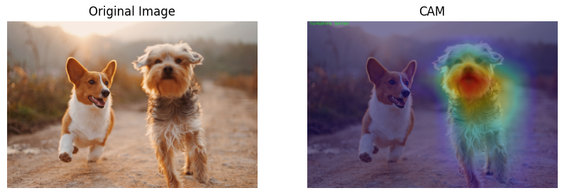
d) Examples of Work:
Here you can see the results of applying CAM to an image of a dogs. The CAM highlights the regions of the image that are most influential in the model’s prediction of the class “Yorkshire Terrier”:
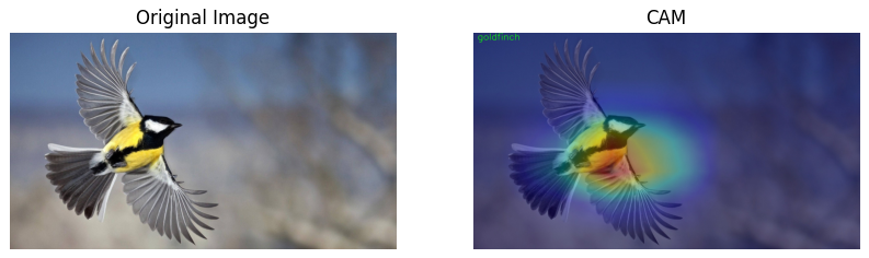
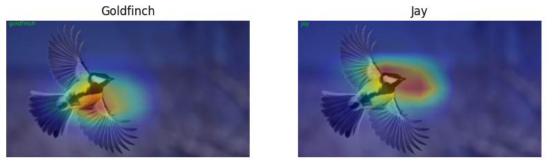
There is another example of applying CAM to an image of a bird:
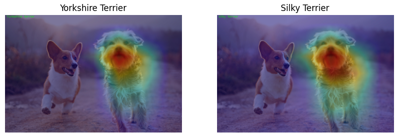
Now let’s see the difference of CAMs for different classes of images.
Section 4: Segmentation - Class Activation Mapping (CAM)
General Definition
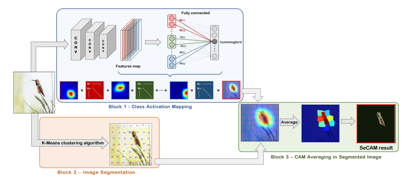
Segmentation-based Class Activation Mapping (SeCAM) is an advanced technique proposed by Quoc Hung Cao, Truong Thanh Hung Nguyen, Vo Thanh Khang Nguyen, and Xuan Phong Nguyen in their paper Segmentation-based Class Activation Mapping. This method combines the principles of Class Activation Mapping (CAM) with image segmentation to provide more interpretable and precise discriminative regions in an image. SeCAM helps in understanding and interpreting the decisions of Convolutional Neural Network (CNN) models by highlighting regions of the image that are most influential in the model’s prediction, segmented into meaningful parts.
How SeCAM Works
a) Steps Involved in SeCAM:
- Feature Extraction:
- Extract the feature maps from the last convolutional layer of the CNN.
- Global Average Pooling (GAP):
- Apply Global Average Pooling (GAP) to the feature maps to get a vector of size equal to the number of feature maps.
- Fully Connected Layer:
- The GAP output is fed into a fully connected layer to get the final class scores.
- Class Activation Mapping (CAM):
- For a given class, compute the weighted sum of the feature maps using the weights from the fully connected layer.
- Superpixel Segmentation:
- Segment the input image into superpixels using the SLIC (Simple Linear Iterative Clustering) algorithm.
- Segmentation-based CAM (SeCAM):
- Combine the CAM values with the segmented superpixels to compute the SeCAM values for each region.
b) SLIC (Simple Linear Iterative Clustering) Algorithm
SLIC is a superpixel segmentation algorithm that clusters pixels in an image into superpixels. Superpixels are contiguous groups of pixels with similar colors or gray levels. The SLIC algorithm adapts k-means clustering to efficiently generate superpixels with uniform size and compactness.
Steps of the SLIC Algorithm
- Initialization:
- Grid Sampling: The image is divided into a grid of $N/K$ equally spaced initial cluster centers, where $N$ is the number of pixels, and $K$ is the desired number of superpixels.
- Perturbation: Each cluster center is moved to the lowest gradient position within a 3x3 neighborhood to avoid placing centers at edges.
- Assignment:
- For each pixel, find the nearest cluster center based on a distance measure that includes color and spatial proximity.
- Distance $D$ is computed as a weighted sum of color distance and spatial distance.
- Update:
- Update each cluster center to the mean of the pixels assigned to it.
- Recompute the cluster centers.
- Enforce Connectivity:
- Ensure that each superpixel is a single connected component.
- Repeat:
- Repeat the assignment and update steps until convergence.
Distance Measure
The distance $D$ between a pixel $i$ and a cluster center $k$ is defined as:
\[D = \sqrt{d_{lab}^2 + \left(\frac{m}{S}\right)^2 d_{xy}^2}\]where:
- $d_{lab}$: Euclidean distance in the CIELAB color space.
- $d_{xy}$: Euclidean distance in the pixel coordinate space.
- $S$: Grid interval, approximately $\sqrt{N/K}$.
- $m$: Compactness parameter, controlling the trade-off between color similarity and spatial proximity.
Numerical Example
Assume we have a small 5x5 grayscale image:
\[\begin{bmatrix} 10 & 10 & 10 & 20 & 20 \\ 10 & 10 & 10 & 20 & 20 \\ 10 & 10 & 10 & 20 & 20 \\ 30 & 30 & 30 & 40 & 40 \\ 30 & 30 & 30 & 40 & 40 \\ \end{bmatrix}\]Let’s apply SLIC to generate 4 superpixels.
- Initialization:
- Number of pixels $N = 25$
- Desired superpixels $K = 4$
- Grid interval $S \approx \sqrt{25 / 4} = 2.5$
- Place initial cluster centers (perturbed for the lowest gradient):
- Cluster Centers = ${ (1, 1), (1, 4), (4, 1), (4, 4) }$
- Assignment:
- For each pixel, compute the distance $D$ to each cluster center.
- Example for pixel at (2,2):
-
Color distance $d_{lab} = 10 - 10 = 0$ - Spatial distance $d_{xy} = \sqrt{(2-1)^2 + (2-1)^2} = \sqrt{2}$
- Assume $m = 10$, $S = 2.5$: \(D = \sqrt{0^2 + \left(\frac{10}{2.5}\right)^2 \cdot 2} = \sqrt{0 + 16 \cdot 2} = \sqrt{32} = 5.66\)
-
- Update:
- Update cluster centers based on the mean of the assigned pixels.
- Recompute centers.
- Enforce Connectivity:
- Ensure all superpixels are connected components.
- Repeat:
- Iterate until convergence.
Output Matrix with Segments:
After applying SLIC, we get the segmented image with superpixels. The output matrix might look like this:
\[\begin{bmatrix} 1 & 1 & 1 & 2 & 2 \\ 1 & 1 & 1 & 2 & 2 \\ 1 & 1 & 1 & 2 & 2 \\ 3 & 3 & 3 & 4 & 4 \\ 3 & 3 & 3 & 4 & 4 \\ \end{bmatrix}\]c) SeCAM Equations
- Feature Maps:
- Let $f_k(x, y)$ represent the activation of unit $k$ in the feature map at spatial location $(x, y)$.
- Class Activation Map (CAM):
- The CAM for class $c$ is computed as: \(M_c(x, y) = \sum_{k} w_{k}^{c} f_k(x, y)\) This gives the importance of each spatial element $(x, y)$ in the feature maps for class $c$.
- SeCAM:
- For each superpixel, the SeCAM value is computed by averaging the CAM values within the superpixel: \(S_c(s) = \frac{1}{|s|} \sum_{(x, y) \in s} M_c(x, y)\) where $|s|$ is the number of pixels in superpixel $s$.
d) Implementation with Code
Step 1-3: Same as for CAM
Step 4: Generate SeCAM
After all preparation steps, we can generate the Segmentation-based Class Activation Maps (SeCAM) for the top K predictions.
def generate_seCAM(feature_maps, softmax_weights, class_indices, segments):
    """
    Generate Segmentation-based Class Activation Maps (SeCAM).
    :param feature_maps: Convolutional feature maps
    :param softmax_weights: Weights of the fully connected layer
    :param class_indices: Class indices
    :param segments: Segmented image regions
    :return: List of SeCAMs for the specified class indices
    """
    batch_size, num_channels, height, width = feature_maps.shape
    output_seCAMs = []

    for class_idx in class_indices:
        cam = softmax_weights[class_idx].dot(feature_maps.reshape((num_channels, height * width)))
        cam = cam.reshape(height, width)
        cam = np.maximum(cam, 0)
        cam = cam / np.max(cam)

        # Resize segments to match cam size
        segments_resized = cv2.resize(segments.astype(np.float32), (width, height), interpolation=cv2.INTER_NEAREST)
        segments_resized = segments_resized.astype(int)

        seCAM = np.zeros_like(cam)
        for seg_val in np.unique(segments_resized):
            mask = (segments_resized == seg_val)
            seCAM[mask] = cam[mask].mean()

        output_seCAMs.append(seCAM)
    return output_seCAMs
batch_size, num_channels, height, width = feature_maps.shape: Retrieves the shape of the feature maps.output_seCAMs = []: Initializes an empty list to store the SeCAMs.for class_idx in class_indices: Iterates over each class index.cam = softmax_weights[class_idx].dot(feature_maps.reshape((num_channels, height * width))): Computes the CAM by taking the weighted sum of the feature maps.cam = cam.reshape(height, width): Reshapes the CAM to the original feature map size.cam = np.maximum(cam, 0): Ensures all CAM values are non-negative.cam = cam / np.max(cam): Normalizes the CAM values to be in the range [0, 1].segments_resized = cv2.resize(segments.astype(np.float32), (width, height), interpolation=cv2.INTER_NEAREST): Resizes the segments to match the CAM size.segments_resized = segments_resized.astype(int): Converts the resized segments to integers.seCAM = np.zeros_like(cam): Initializes an array of zeros with the same shape as the CAM.for seg_val in np.unique(segments_resized): Iterates over each unique segment value.mask = (segments_resized == seg_val): Creates a mask for the current segment.seCAM[mask] = cam[mask].mean(): Assigns the mean CAM value of the current segment to the SeCAM array.output_seCAMs.append(seCAM): Adds the SeCAM to the list of output SeCAMs.
This function generates Segmentation-based CAMs (SeCAMs) by combining CAM values with superpixel segments, resulting in more interpretable and precise discriminative regions.
Step 5: Display and Save SeCAM
After generating the SeCAMs, we can overlay them on the original image, mask insignificant regions, and display the results.
def display_and_save_seCAM(SeCAMs, width, height, original_image, save_name, secam_threshold, plot=True):
    """
    Display and save the SeCAM images.
    :param SeCAMs: List of SeCAMs
    :param width: Width of the original image
    :param height: Height of the original image
    :param original_image: Original input image
    :param save_name: Name to save the output image
    :param secam_threshold: Threshold to mask significant regions
    :param plot: Whether to display the image
    """
    matplotlib.rcParams['figure.figsize'] = 15, 12

    for i, seCAM in enumerate(SeCAMs):
        seCAM = np.uint8(255 * seCAM)
        seCAM_resized = cv2.resize(seCAM, (width, height))

        # Create a mask of the significant regions
        mask = seCAM_resized > (secam_threshold * seCAM_resized.max())

        # Create a black background image
        black_bg = np.zeros_like(original_image)

        # Apply the mask to the original image
        result = original_image.copy()
        result[~mask] = black_bg[~mask]

        # Save the result
        cv2.imwrite(f"outputs/SeCAM_{save_name}_{i}.jpg", result)

        # Display the result
        if plot:
            image = plt.imread(f"outputs/SeCAM_{save_name}_{i}.jpg")
            plt.imshow(image)
            plt.axis('off')
            plt.show()
matplotlib.rcParams['figure.figsize'] = 15, 12: Sets the figure size for matplotlib plots.for i, seCAM in enumerate(SeCAMs): Iterates over each SeCAM.seCAM = np.uint8(255 * seCAM): Scales the SeCAM values to the range [0, 255] and converts them to uint8 format.seCAM_resized = cv2.resize(seCAM, (width, height)): Resizes the SeCAM to match the original image size.mask = seCAM_resized > (secam_threshold * seCAM_resized.max()): Creates a mask for significant regions in the SeCAM.black_bg = np.zeros_like(original_image): Creates a black background image.result = original_image.copy(): Copies the original image.result[~mask] = black_bg[~mask]: Applies the mask to the original image, keeping only the significant regions.cv2.imwrite(f"outputs/SeCAM_{save_name}_{i}.jpg", result): Saves the result image.image = plt.imread(f"outputs/SeCAM_{save_name}_{i}.jpg"): Reads the saved image.plt.imshow(image): Displays the image.plt.axis('off'): Hides the axis.plt.show(): Shows the image.
This function overlays the SeCAM on the original image, masks insignificant regions, adds the class label, and saves the result. It also displays the final image.
Step 3: Full Pipeline for Generating and Saving SeCAM
Finally, we can combine all the above steps into a single function to generate and save SeCAMs for the top K predictions of an input image.
def generate_and_save_seCAM(image_path, topk_predictions, num_segments=50, compactness=10, secam_threshold=0.8):
    """
    Generate and save SeCAM for the specified image and topk predictions.
    :param image_path: Path to the input image
    :param topk_predictions: Number of top predictions to generate SeCAM for
    :param num_segments: Number of segments for SLIC
    :param compactness: Compactness parameter for SLIC
    :param secam_threshold: Threshold to mask significant regions in SeCAM
    """
    # Load the class labels
    class_labels = load_class_labels('LOC_synset_mapping.txt')

    # Read and preprocess the image
    image_tensor, original_image, height, width = preprocess_image(image_path)

    # Load the model and extract features
    model, features_blobs, softmax_weights = load_model_and_extract_features()

    # Get the top k predictions
    class_indices = get_topk_predictions(model, image_tensor, topk_predictions)

    # Generate superpixels using SLIC
    segments = slic(original_image, n_segments=num_segments, compactness=compactness, start_label=1)

    # Generate SeCAM for the top predictions
    SeCAMs = generate_seCAM(features_blobs[0], softmax_weights, class_indices, segments)

    # Display and save the SeCAM results
    save_name = image_path.split('/')[-1].split('.')[0] + f"_seg_{num_segments}_ts_{secam_threshold}"
    display_and_save_seCAM(SeCAMs, width, height, original_image, save_name, secam_threshold)
class_labels = load_class_labels('LOC_synset_mapping.txt'): Loads the class labels from a specified file.image_tensor, original_image, height, width = preprocess_image(image_path): Reads and preprocesses the input image, returning the preprocessed image tensor, original image, and image dimensions.model, features_blobs, softmax_weights = load_model_and_extract_features(): Loads the model and extracts the feature maps and softmax weights.class_indices, _ = get_topk_predictions(model, image_tensor, topk_predictions): Gets the top K predictions for the input image.segments = slic(original_image, n_segments=num_segments, compactness=compactness, start_label=1): Segments the input image into superpixels using the SLIC algorithm.SeCAMs = generate_seCAM(features_blobs[0], softmax_weights, class_indices, segments): Generates the SeCAMs for the top predictions.save_name = image_path.split('/')[-1].split('.')[0]: Extracts the base name of the image file for saving the results.display_and_save_seCAM(SeCAMs, width, height, original_image, class_indices, class_labels, save_name, secam_threshold): Displays and saves the SeCAM results.
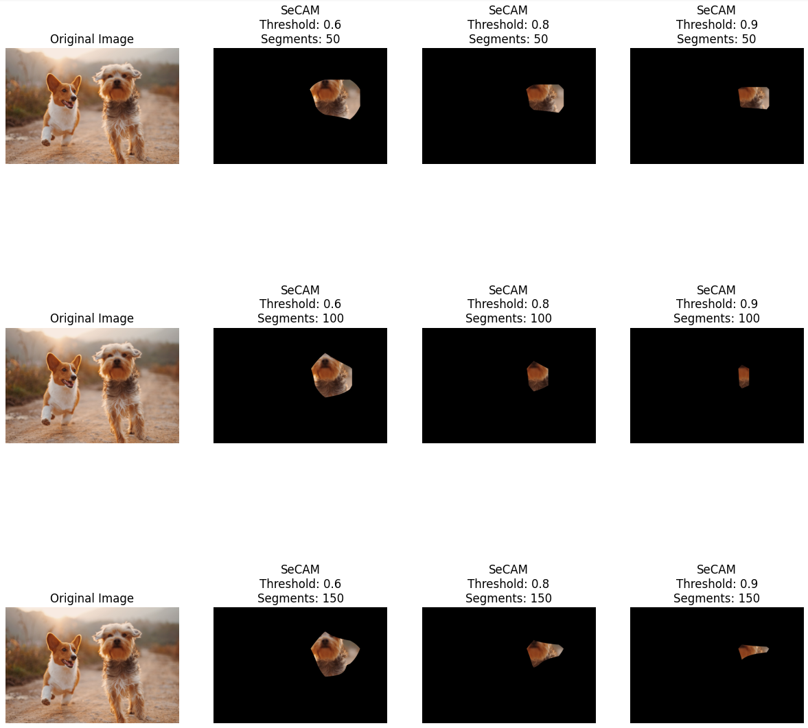
e) Examples of Work:
Here you can see the results of applying SeCAM to an image of a dogs using different number of segments and threshold values:
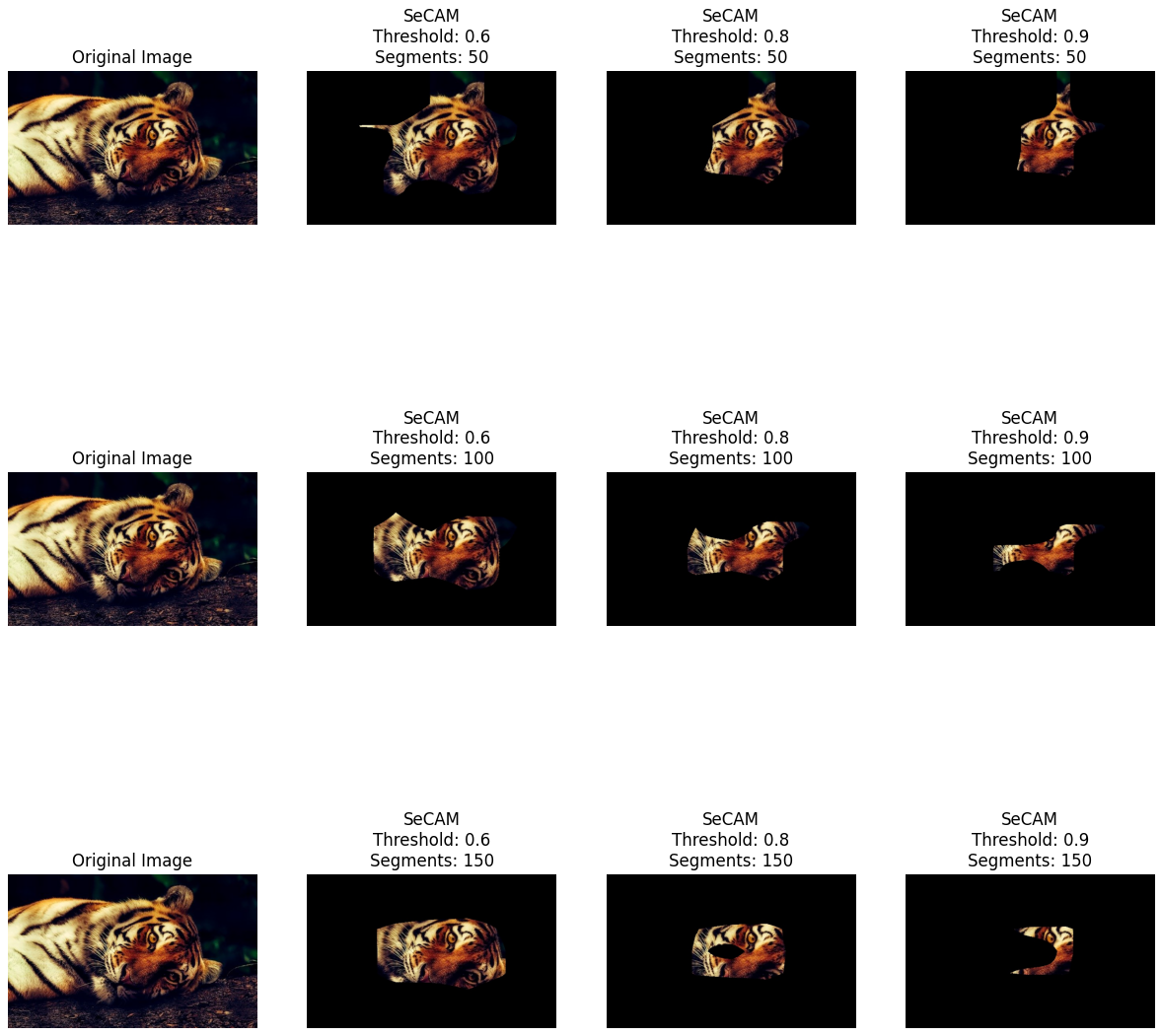
There is another example of applying SeCAM to an image of a tiger:
Conclusion
In this tutorial, we have explored the concepts of Class Activation Mapping (CAM) and Segmentation-based Class Activation Mapping (SeCAM) as Explainable AI (XAI) methods for understanding image classification models. We have seen how CAM highlights discriminative regions in an image that contribute to the model’s prediction and how SeCAM combines CAM with image segmentation to provide more interpretable and precise results. By visualizing the CAM and SeCAM results, we can gain insights into the decision-making process of Convolutional Neural Networks and understand the basis of their predictions. These XAI methods play a crucial role in making AI models more transparent, interpretable, and trustworthy in critical applications where human understanding is essential.